KI (Künstliche Intelligenz, aka AI) mit Python, tensorflow und keras

Ziel der hier vorgestellten Script-Lösung: Ein neuronales Netz wird aufgebaut und mit den Bildern einer freien Bilddatenbank trainiert. Dabei umfasst die von cifar10 gewählte Datenbank Bilder aus den Rubriken "Flugzeug", "Auto", "Vogel", "Katze", "Reh", "Hund", "Frosch", "Pferd", "Schiff" und "LKW". Nach dem Training werden dem Netz eigene Bilder vorgelegt, in denen das NeuroNetz bekannte Objekte (gemäß gelernter features) identifizieren soll.

Zuerst wird der Bestand einer Bilddatenbank via cifar10 geladen und der Datenbestand ggf. reduziert:

# fetch cifar10-images:
(training_images, training_label) , (testing_images, testing_label) = datasets.cifar10.load_data()

#training_images = training_images[:20000]
#training_label = training_label[:20000]
#testing_images = testing_images[:2000]
#testing_label = testing_label[:2000]

Anschliessend wird das Neuronale Netz aufgebaut (model = models.Sequential()) Danach folgt die Angabe der kaskadierten Filter, die nacheinander geschaltet sind, beginnend mit einem Convolutional Layer, der die 32*32-Pixel images hält, bis hin zum finalen Dense-Layer mit 10 Neuronen und der Softmax-Funktion.

# Sequential Neural Network:
model = models.Sequential()

# And now, the cascades filters of our network, starting with a Convolutional Layer
# relu = rectified linear unit, or: f(x) = max(0, x)
# Convolutional Layer consisting of 32 filters with 3x3 matrixes, shape of 32x32-images with RGB-colors:
model.add(layers.Conv2D(32, (3,3), activation = 'relu', input_shape = (32, 32, 3)))
model.add(layers.MaxPooling2D((2, 2)))
model.add(layers.Conv2D(64, (3,3), activation = 'relu'))
model.add(layers.MaxPooling2D((2, 2)))
model.add(layers.Conv2D(64, (3,3), activation = 'relu'))
model.add(layers.Flatten())
model.add(layers.Dense(64, activation = 'relu'))    # 64 neurons
model.add(layers.Dense(10, activation = 'softmax')) # 10 neurons, softmax gives procentual values

Nach der Definition des Netzwerks erfolgt dessen Compilierung, dann dessen Training. Zum Training wird das Bildmaterial 'epochs'-mal dem Netzwerk präsentiert.

# compile with Adam Optimizer and use 'Sparse Categorical Crossentropy' as Loss function:
model.compile(optimizer = 'adam', loss = 'sparse_categorical_crossentropy', metrics = ['accuracy'])

# apply data 22 times at the model (epochs) to improve accurancy:
model.fit(training_images, training_label, epochs = 22, validation_data = (testing_images, testing_label))

Auf stderr kann man das Training nach verfolgen und dabei die Zunahme der Akkuratesse erkennen.

compile, train and test neuro network
Epoch 1/22
1563/1563 [==============================] - 30s 19ms/step - loss: 1.5239 - accuracy: 0.4438 - val_accuracy: 0.5467 - val_loss: 1.2610
Epoch 2/22
1563/1563 [==============================] - 30s 19ms/step - loss: 1.1611 - accuracy: 0.5895 - val_accuracy: 0.6284 - val_loss: 1.0483
Epoch 3/22
1563/1563 [==============================] - 29s 19ms/step - loss: 1.0166 - accuracy: 0.6454 - val_accuracy: 0.6305 - val_loss: 1.0500
Epoch 4/22
1563/1563 [==============================] - 30s 19ms/step - loss: 0.9271 - accuracy: 0.6753 - val_accuracy: 0.6726 - val_loss: 0.9469
Epoch 5/22
1563/1563 [==============================] - 23s 15ms/step - loss: 0.8552 - accuracy: 0.6980 - val_accuracy: 0.6738 - val_loss: 0.9305
Epoch 6/22
1563/1563 [==============================] - 23s 15ms/step - loss: 0.7972 - accuracy: 0.7192 - val_accuracy: 0.6831 - val_loss: 0.9180
Epoch 7/22
1563/1563 [==============================] - 26s 17ms/step - loss: 0.7475 - accuracy: 0.7378 - val_accuracy: 0.7073 - val_loss: 0.8500
Epoch 8/22
1563/1563 [==============================] - 23s 15ms/step - loss: 0.7063 - accuracy: 0.7513 - val_accuracy: 0.6963 - val_loss: 0.8900
Epoch 9/22
1563/1563 [==============================] - 23s 14ms/step - loss: 0.6685 - accuracy: 0.7635 - val_accuracy: 0.6813 - val_loss: 0.9468
Epoch 10/22
1563/1563 [==============================] - 23s 14ms/step - loss: 0.6301 - accuracy: 0.7756 - val_accuracy: 0.7074 - val_loss: 0.8841
Epoch 11/22
1563/1563 [==============================] - 23s 15ms/step - loss: 0.5977 - accuracy: 0.7878 - val_accuracy: 0.7162 - val_loss: 0.8579

Interessant ist auch, sowohl mit dem epochs-Wert als auch mit der Anzahl verwendeter Bilder zu spielen. Wichtiger als die Auswirkungen auf die Laufzeit ist die funktionale Wirkung. Man sehe sich z.B. das Ergebnis mit epochs=1 (accuracy=0.44) an - da wird aus einem Pony (Pferd) gerne mal ein Vogel.

Als letztes werden n eigene Bilder dem Netzwerk vorgelegt, die daraus resultierende prediction gibt an, welcher Klasse das eigene Bild zugeordnet wurde.
Die Bilder:

# let's detect own photos by the neuro network:
for prefix in ['petra_and_pops', 'pops_front', 'sunny']:
    pic = prefix + '_32_32.jpg'
    print("operating %s" % (pic))
    image = cv.imread(pic)
    image = cv.cvtColor(image, cv.COLOR_BGR2RGB)

    #plt.imshow(image, cmap = plt.cm.binary)
    #plt.show()

    prediction = model.predict(np.array([image]) / 255)
    index = np.argmax(prediction)
    print(classes[index])

Das Ergebnis auf der shell:

operating petra_and_pops_32_32.jpg
Pferd
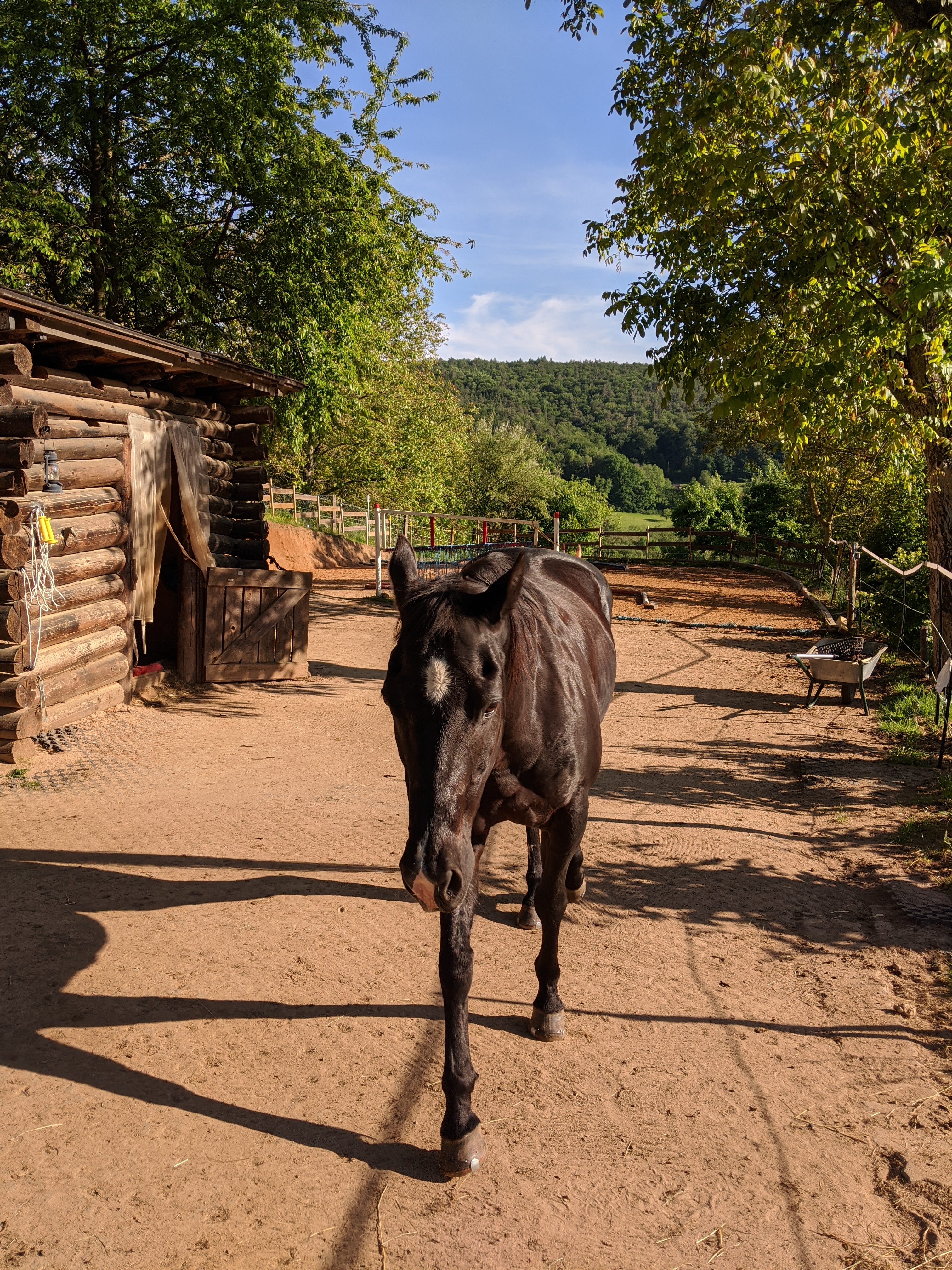
operating pops_front_32_32.jpg
Pferd
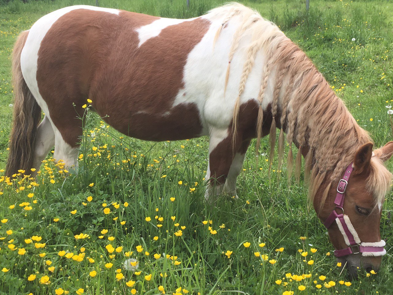
operating sunny_32_32.jpg
Pferd
done

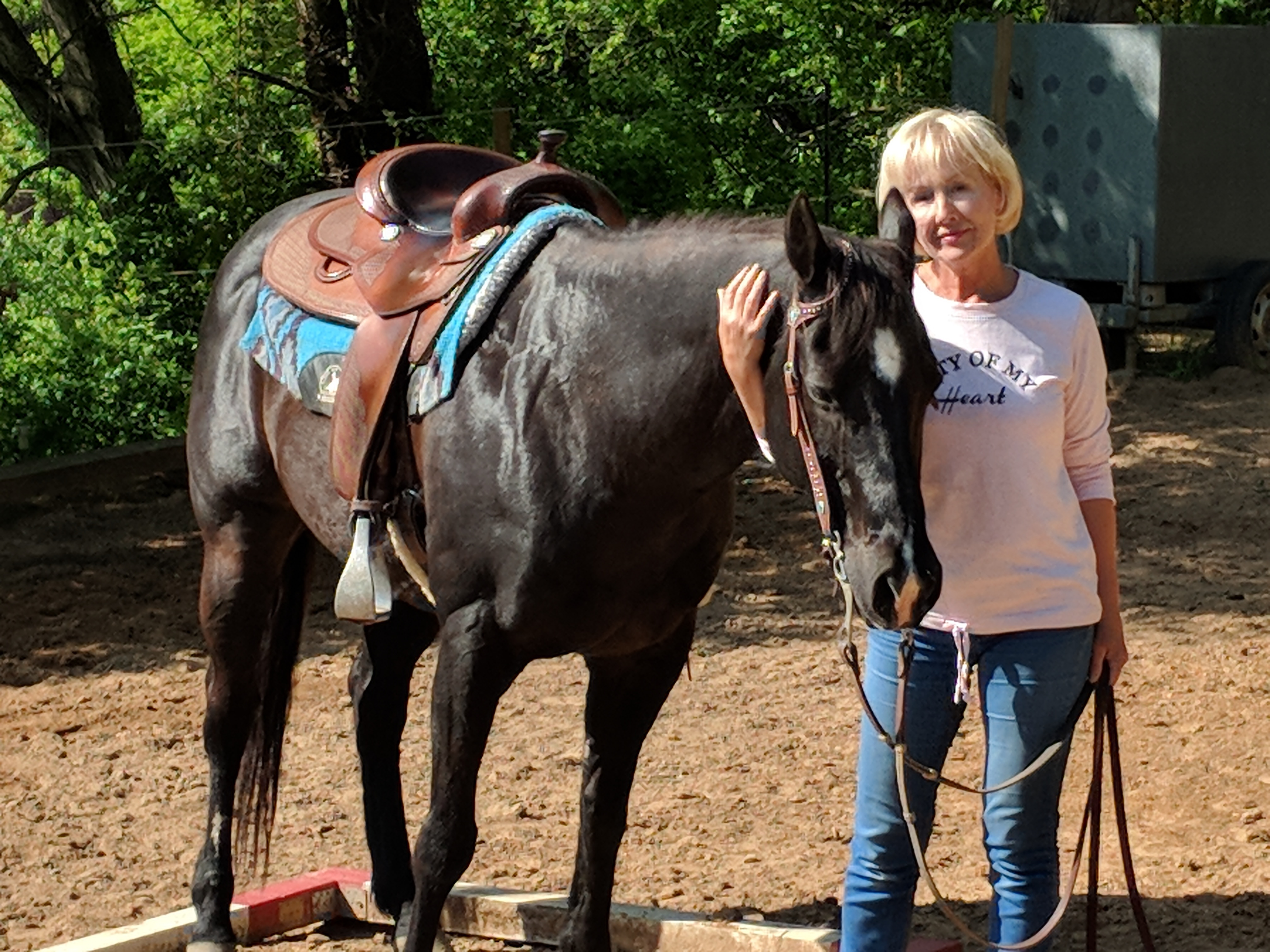
(Das erste Bild liefert nur das Pferd, da die Klasse 'Mensch' im gelernten Datenbestand nicht enthalten war.)

Wer ein kindle besitzt, findet im kindle-store das kostenlose eBook "Python für neuronale Netze; der schnelle Einstieg" von Florian Dedov, dass vielerlei Stoff bietet.

Bevor das Script laufen kann, muss man ggf. verschiedene Python-Pakete installieren. Für TensorFlow bietet sich die Sequenz

• pip install -U pip
• pip install -U setuptools
• pip3 install TensorFlow oder: pip3 install tf-nightly

#!/usr/bin/env python3 # # t1.py # # to install TensorFlow: # pip install -U pip # pip install -U setuptools # # pip3 install tf-nightly # import cv2 as cv import numpy as np import matplotlib.pyplot as plt from tensorflow.keras import datasets, layers, models # fetch cifar10-images: (training_images, training_label) , (testing_images, testing_label) = datasets.cifar10.load_data() # uncopmment lines below to improve speed by q-loss: #training_images = training_images[:20000] #training_label = training_label[:20000] #testing_images = testing_images[:2000] #testing_label = testing_label[:2000] # normalize colors to a range from 0.0 to 1.0: training_images, testing_images = training_images / 255.0, testing_images / 255.0 # names of the categories provided by the cifar10-fetch: classes = ['Flugzeug', 'Auto', 'Vogel', 'Katze', 'Reh', 'Hund', 'Frosch', 'Pferd', 'Schiff', 'LKW'] # display images of the classes: #for i in range(16): # plt.subplot(4, 4, i + 1) # plt.xticks([]) # plt.yticks([]) # plt.imshow(training_images[i], cmap=plt.cm.binary) # plt.xlabel(classes[training_label[i][0]]) # #plt.show() print("build up neuro network") # Sequential Neural Network: model = models.Sequential() # And now, the cascades filters of our network, starting with a Convolutional Layer # relu = rectified linear unit, or: f(x) = max(0, x) # Convolutional Layer consisting of 32 filters with 3x3 matrixes, shape of 32x32-images with RGB-colors: model.add(layers.Conv2D(32, (3,3), activation = 'relu', input_shape = (32, 32, 3))) model.add(layers.MaxPooling2D((2, 2))) model.add(layers.Conv2D(64, (3,3), activation = 'relu')) model.add(layers.MaxPooling2D((2, 2))) model.add(layers.Conv2D(64, (3,3), activation = 'relu')) model.add(layers.Flatten()) model.add(layers.Dense(64, activation = 'relu')) # 64 neurons model.add(layers.Dense(10, activation = 'softmax')) # 10 neurons, softmax gives procentual values print("compile, train and test neuro network") # compile with Adam Optimizer and use 'Sparse Categorical Crossentropy' as Loss function: model.compile(optimizer = 'adam', loss = 'sparse_categorical_crossentropy', metrics = ['accuracy']) # apply data 22 times at the model (epochs) to improve accurancy: model.fit(training_images, training_label, epochs = 22, validation_data = (testing_images, testing_label)) testing_loss, testing_acc = model.evaluate(testing_images, testing_label, verbose = 2) # let's detect own photos by the neuro network: for prefix in ['petra_and_pops', 'pops_front', 'sunny']: pic = prefix + '_32_32.jpg' print("operating %s" % (pic)) image = cv.imread(pic) image = cv.cvtColor(image, cv.COLOR_BGR2RGB) #plt.imshow(image, cmap = plt.cm.binary) #plt.show() prediction = model.predict(np.array([image]) / 255) index = np.argmax(prediction) print(classes[index]) print("done")